
Trace-based metrics
WARNING: This page describes the legacy (v1) metric system. For all new use cases, please refer to the Trace Summarization documentation, which is the successor to this system. This page is only kept around as a historical reference.
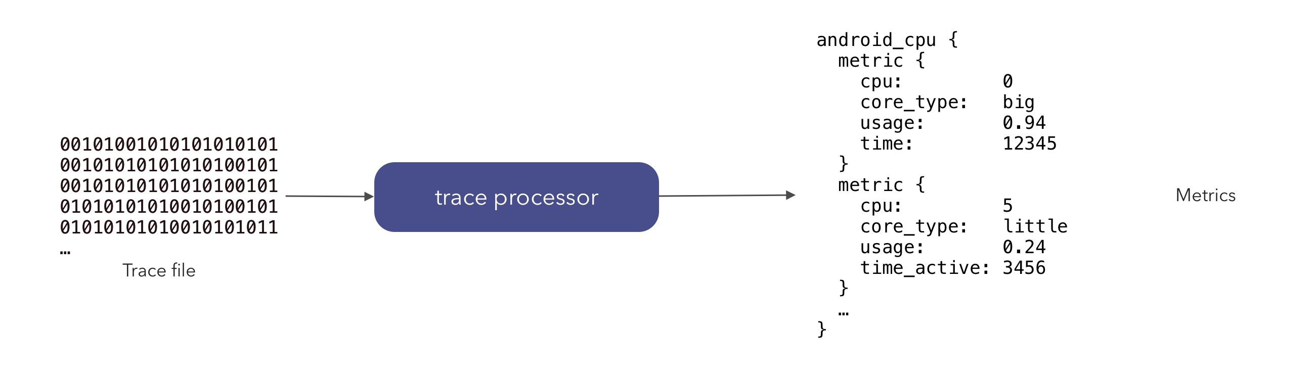
The metrics subsystem is a part of the trace processor which uses traces to compute reproducible metrics. It can be used in a wide range of situations; examples include benchmarks, lab tests and on large corpuses of traces.
Introduction
Motivation
Performance metrics are useful to monitor for the health of a system and ensure that a system does not regress over time as new features are added.
However, metrics retrieved directly from the system have a downside: if there is a regression, it is difficult to root-cause the issue. Often, the problem may not be reproducible or may rely on a particular setup.
Trace-based metrics are one possible solution to this problem. Instead of collecting metrics directly on the system, a trace is collected and metrics are computed from the trace. If a regression in the metric is spotted, the developer can look directly at the trace to understand why the regression has occurred instead of having to reproduce the issue.
Metric subsystem
The metric subsystem is a part of the trace processor which executes SQL queries against traces and produces a metric which summarizes some performance attribute (e.g. CPU, memory, startup latency etc.).
For example, generating the Android CPU metrics on a trace is as simple as:
> ./trace_processor --run-metrics android_cpu <trace>
android_cpu {
  process_info {
    name: "/system/bin/init"
    threads {
      name: "init"
      core {
        id: 1
        metrics {
          mcycles: 1
          runtime_ns: 570365
          min_freq_khz: 1900800
          max_freq_khz: 1900800
          avg_freq_khz: 1902017
        }
      }
      ...
    }
    ...
  }
  ...
}
Metric development guide
As metric writing requires a lot of iterations to get right, there are several tips which make the experience a lot smoother.
Hot reloading metrics
To obtain the fastest possible iteration time when developing metrics, it's possible to hot reload any changes to SQL; this will skip over both recompilation (for builtin metrics) and trace load (for both builtin and custom metrics).
To do this, trace processor is started in interactive mode while still
specifying command line flags about which metrics should be run and the paths of
any extensions. Then, in the REPL shell, the commands .load-metrics-sql (which
causes any SQL on disk to be re-read) and .run-metrics (to run the metrics and
print the result).
For example, suppose we want to iterate on the android_startup metric. We can
run the following commands from a Perfetto checkout:
> ./tools/trace_processor --interactive \
  --run-metrics android_startup \
  --metric-extension src/trace_processor/metrics@/ \
  --dev \
  <trace>
android_startup {
  <contents of startup metric>
}

# Now make any changes you want to the SQL files related to the startup
# metric. Even adding new files in the src/trace_processor/metric works.

# Then, we can reload the changes using `.load-metrics-sql`.
> .load-metrics-sql

# We can rerun the changed metric using `.run-metrics`
> .run-metrics
android_startup {
  <contents of changed startup metric>
}
NOTE: see below about why --dev was required for this command.
This also works for custom metrics specified on the command line:
> ./tools/trace_processor -i --run-metrics /tmp/my_custom_metric.sql <trace>
my_custom_metric {
  <contents of my_custom_metric>
}

# Change the SQL file as before.

> .load-metrics-sql
> .run-metrics
my_custom_metric {
  <contents of changed my_custom_metric>
}
WARNING: it is currently not possible to reload protos in the same way. If protos are changed, a recompile (for built-in metrics) and reinvoking trace processor is necessary to pick up the changes.
WARNING: Deleted files from --metric-extension folders are not removed and
will remain available e.g. to RUN_METRIC invocations.
Modifying built-in metric SQL without recompiling
It is possible to override the SQL of built-in metrics at runtime without
needing to recompile trace processor. To do this, the flag --metric-extension
needs to be specified with the disk path where the built-metrics live and the
special string / for the virtual path.
For example, from inside a Perfetto checkout:
> ./tools/trace_processor \
  --run-metrics android_cpu \
  --metric-extension src/trace_processor/metrics@/
  --dev
  <trace>
This will run the CPU metric using the live SQL in the repo not the SQL definition built into the binary.
NOTE: protos are not overridden in the same way - if any proto messages are changed a recompile of trace processor is required for the changes to be available.
NOTE: the --dev flag is required for the use of this feature. This flag
ensures that this feature is not accidentally in production as it is only
intended for local development.
WARNING: protos are not overridden in the same way - if any proto messages are changed a recompile of trace processor is required for the changes to be available.
Metric helper functions
RUN_METRIC
RUN_METRIC allows you to run another metric file. This allows you to use views
or tables defined in that file without repetition.
Conceptually, RUN_METRIC adds composability for SQL queries to break a big
SQL metric into smaller, reusable files. This is similar to how functions allow
decomposing large chunks in traditional programming languages.
A simple usage of RUN_METRIC would be as follows:
In file android/foo.sql:
CREATE VIEW view_defined_in_foo AS
SELECT *
FROM slice
LIMIT 1;
In file android/bar.sql
SELECT RUN_METRIC('android/foo.sql');

CREATE VIEW view_depending_on_view_from_foo AS
SELECT *
FROM view_defined_in_foo
LIMIT 1;
RUN_METRIC also supports running templated metric files. Here's an example
of what that looks like:
In file android/slice_template.sql:
CREATE VIEW {{view_name}} AS
SELECT *
FROM slice
WHERE slice.name = '{{slice_name}}';
In file android/metric.sql:
SELECT RUN_METRIC(
  'android/slice_template.sql',
  'view_name', 'choreographer_slices',
  'slice_name', 'Chroeographer#doFrame'
);

CREATE VIEW long_choreographer_slices AS
SELECT *
FROM choreographer_slices
WHERE dur > 1e6;
When running slice_template.sql, trace processor will substitute the arguments
passed to RUN_METRIC into the templated file before executing the file using
SQLite.
In other words, this is what SQLite sees and executes in practice for the above example:
CREATE VIEW choreographer_slices AS
SELECT *
FROM slice
WHERE slice.name = 'Chroeographer#doFrame';

CREATE VIEW long_choreographer_slices AS
SELECT *
FROM choreographer_slices
WHERE dur > 1e6;
The syntax for templated metric files is essentially a highly simplified version of Jinja's syntax.
Walkthrough: prototyping a metric
TIP: To see how to add a new metric to trace processor, see the checklist here
This walkthrough will outline how to prototype a metric locally without needing to compile trace processor. This metric will compute the CPU time for every process in the trace and list the names of the top 5 processes (by CPU time) and the number of threads created by the process.
NOTE: See this GitHub gist to see how the code should look at the end of the walkthrough. The prerequisites and Step 4 below give instructions on how to get trace processor and run the metrics code.
Prerequisites
As a setup step, create a folder to act as a scratch workspace; this folder will
be referred to using the env variable $WORKSPACE in Step 4.
The other requirement is trace processor. This can downloaded from here or can be built from source using the instructions here. Whichever method is chosen, $TRACE_PROCESSOR env variable will be used to refer to the location of the binary in Step 4.
Step 1
As all metrics in the metrics platform are defined using protos, the metric needs to be structured as a proto. For this metric, there needs to be some notion of a process name along with its CPU time and number of threads.
Starting off, in a file named top_five_processes.proto in our workspace,
create a basic proto message called ProcessInfo with those three fields:
message ProcessInfo {
  optional string process_name = 1;
  optional uint64 cpu_time_ms = 2;
  optional uint32 num_threads = 3;
}
Next , create a wrapping message which will hold the repeated field containing the top 5 processes.
message TopProcesses {
  repeated ProcessInfo process_info = 1;
}
Finally, define an extension to the root proto for all metrics (the TraceMetrics proto).
extend TraceMetrics {
  optional TopProcesses top_five_processes = 450;
}
Adding this extension field allows trace processor to link the newly defined
metric to the TraceMetrics proto.
Notes:
- The field ids 450-500 are reserved for local development so any of them can be used as the field id for the extension field.
- The choice of field name here is important as the SQL file and the final table generated in SQL will be based on this name.
Putting everything together, along with some boilerplate preamble gives:
syntax = "proto2";

package perfetto.protos;

import "protos/perfetto/metrics/metrics.proto";

message ProcessInfo {
  optional string process_name = 1;
  optional int64 cpu_time_ms = 2;
  optional uint32 num_threads = 3;
}

message TopProcesses {
  repeated ProcessInfo process_info = 1;
}

extend TraceMetrics {
  optional TopProcesses top_five_processes = 450;
}
Step 2
Next, write the SQL to generate the table of the top 5 processes ordered by the sum of the CPU time they ran for and the number of threads which were associated with the process.
The following SQL should be added to a file called top_five_processes.sql in
the workspace:
CREATE VIEW top_five_processes_by_cpu AS
SELECT
  process.name as process_name,
  CAST(SUM(sched.dur) / 1e6 as INT64) as cpu_time_ms,
  COUNT(DISTINCT utid) as num_threads
FROM sched
INNER JOIN thread USING(utid)
INNER JOIN process USING(upid)
GROUP BY process.name
ORDER BY cpu_time_ms DESC
LIMIT 5;
Let's break this query down:
- The first table used is the
schedtable. This contains all the scheduling data available in the trace. Each scheduling "slice" is associated with a thread which is uniquely identified in Perfetto traces using itsutid. The two pieces of information needed from the sched table are thedur- short for duration, this is the amount of time the slice lasted - and theutidwhich will be used to join with the thread table. - The next table is the thread table. This gives us a lot of information which
is not particularly interesting (including its thread name) but it does give
us the
upid. Similar toutid,upidis the unique identifier for a process in a Perfetto trace. In this case,upidwill refer to the process which hosts the thread given byutid. - The final table is the process table. This gives the name of the process associated with the original sched slice.
- With the process, thread and duration for each sched slice, all the slices for a single processes are collected and their durations summed to get the CPU time (dividing by 1e6 as sched's duration is in nanoseconds) and the number of distinct threads.
- Finally, we order by the cpu time and limit to the top 5 results.
Step 3
Now that the result of the metric has been expressed as an SQL table, it needs to be converted to a proto. The metrics platform has built-in support for emitting protos using SQL functions; something which is used extensively in this step.
Let's look at how it works for our table above.
CREATE VIEW top_five_processes_output AS
SELECT TopProcesses(
  'process_info', (
    SELECT RepeatedField(
      ProcessInfo(
        'process_name', process_name,
        'cpu_time_ms', cpu_time_ms,
        'num_threads', num_threads
      )
    )
    FROM top_five_processes_by_cpu
  )
);
Breaking this down again:
Starting from the inner-most SELECT statement, there is what looks like a function call to the ProcessInfo function; in fact this is no coincidence. For each proto that the metrics platform knows about, an SQL function is generated with the same name as the proto. This function takes key value pairs with the key as the name of the proto field to fill and the value being the data to store in the field. The output is the proto created by writing the fields described in the function. (*)
In this case, this function is called once for each row in the
top_five_processes_by_cputable. The output will be the fully filled ProcessInfo proto.The call to the
RepeatedFieldfunction is the most interesting part and also the most important. In technical terms,RepeatedFieldis an aggregate function. Practically, this means that it takes a full table of values and generates a single array which contains all the values passed to it.Therefore, the output of this whole SELECT statement is an array of 5 ProcessInfo protos.
Next is creation of the
TopProcessesproto. By now, the syntax should already feel somewhat familiar; the proto builder function is called to fill in theprocess_infofield with the array of protos from the inner function.The output of this SELECT is a single
TopProcessesproto containing the ProcessInfos as a repeated field.Finally, the view is created. This view is specially named to allow the metrics platform to query it to obtain the root proto for each metric (in this case
TopProcesses). See the note below as to the pattern behind this view's name.
(*) This is not strictly true. To type-check the protos, some metadata is returned about the type of the proto but this is unimportant for metric authors.
NOTE: It is important that the views be named {name of TraceMetrics extension field}_output. This is the pattern used and expected by the metrics platform for all metrics.
The final file should look like so:
CREATE VIEW top_five_processes_by_cpu AS
SELECT
  process.name as process_name,
  CAST(SUM(sched.dur) / 1e6 as INT64) as cpu_time_ms,
  COUNT(DISTINCT utid) as num_threads
FROM sched
INNER JOIN thread USING(utid)
INNER JOIN process USING(upid)
GROUP BY process.name
ORDER BY cpu_time_ms DESC
LIMIT 5;

CREATE VIEW top_five_processes_output AS
SELECT TopProcesses(
  'process_info', (
    SELECT RepeatedField(
      ProcessInfo(
        'process_name', process_name,
        'cpu_time_ms', cpu_time_ms,
        'num_threads', num_threads
      )
    )
    FROM top_five_processes_by_cpu
  )
);
NOTE: The name of the SQL file should be the same as the name of TraceMetrics extension field. This is to allow the metrics platform to associated the proto extension field with the SQL which needs to be run to generate it.
Step 4
TRACE_PROCESSOR --run-metrics $WORKSPACE/top_five_processes.sql $TRACE 2> /dev/null(For an example trace to test this on, see the Notes section below.)
By passing the SQL file for the metric to be computed, trace processor uses the
name of this file to find the proto and to figure out the name of the output
table for the proto and the name of the extension field for TraceMetrics; this
is the reason it was important to choose the names of these other objects
carefully.
Notes:
- If something doesn't work as intended, check that the workspace looks the same as the contents of this GitHub gist.
- A good example trace for this metric is the Android example trace used by the Perfetto UI found here.
- stderr is redirected to remove any noise from parsing the trace that trace processor generates.
If everything went successfully, the following output should be visible (specifically this is the output for the Android example trace linked above):
[perfetto.protos.top_five_processes] {
  process_info {
    process_name: "com.google.android.GoogleCamera"
    cpu_time_ms: 15154
    num_threads: 125
  }
  process_info {
    process_name: "sugov:4"
    cpu_time_ms: 6846
    num_threads: 1
  }
  process_info {
    process_name: "system_server"
    cpu_time_ms: 6809
    num_threads: 66
  }
  process_info {
    process_name: "cds_ol_rx_threa"
    cpu_time_ms: 6684
    num_threads: 1
  }
  process_info {
    process_name: "com.android.chrome"
    cpu_time_ms: 5125
    num_threads: 49
  }
}
Next steps
- The common tasks page gives a list of steps on how new metrics can be added to the trace processor.
Appendix: Case for upstreaming
NOTE: Googlers: for internal usage of metrics in Google3 (i.e. metrics which are confidential), please see this internal page.
Authors are strongly encouraged to add all metrics derived on Perfetto traces to the Perfetto repo unless there is a clear usecase (e.g. confidentiality) why these metrics should not be publicly available.
In return for upstreaming metrics, authors will have first class support for running metrics locally and the confidence that their metrics will remain stable as trace processor is developed.
As well as scaling upwards while developing from running on a single trace locally to running on a large set of traces, the reverse is also very useful. When an anomaly is observed in the metrics of a lab benchmark, a representative trace can be downloaded and the same metric can be run locally in trace processor.
Since the same code is running locally and remotely, developers can be confident in reproducing the issue and use the trace processor and/or the Perfetto UI to identify the problem.