
heapprofd: Sampling for Memory Profiles
tomlewin, fmayer · 2021-04-14
Background
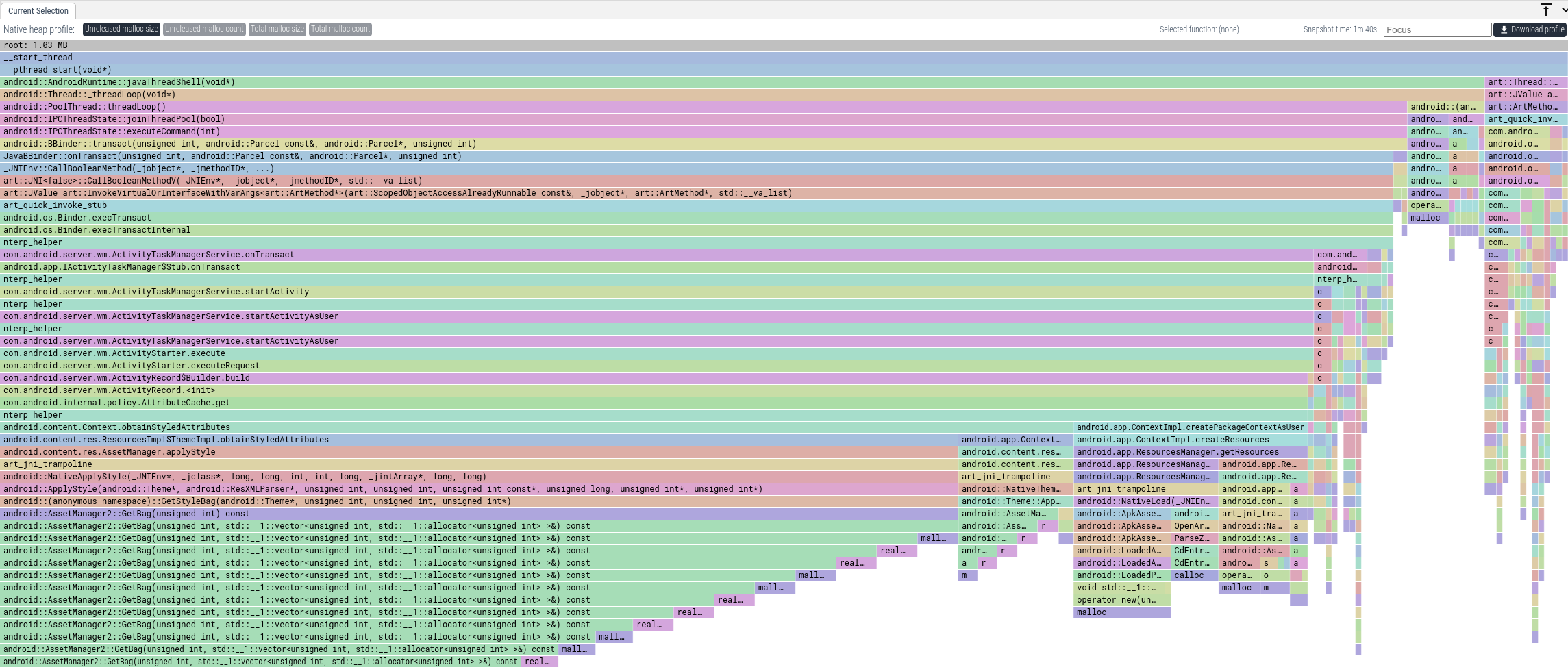
A heap profiler associates memory allocations with the callstacks on which they happen (example visualization). It is prohibitively expensive to handle every allocation done by a program, so the Android Heap Profiler employs a sampling approach that handles a statistically meaningful subset of allocations. This document explores the statistical properties thereof.
Conceptual motivation
Conceptually the sampling is implemented such that each byte has some probability p of being sampled. In theory we can think of each byte undergoing a Bernoulli trial. The reason we use a random sampling approach, as opposed to taking every nth byte, is that there may be regular allocation patterns in the code that may be missed by a correspondingly regular sampling.
To scale the sampled bytes to the correct scale, we multiply by 1 / p, i.e. if we sample a byte with probability 10%, then each byte sampled represents 10 bytes allocated.
Implementation
In practice, the algorithm works as follows:
We look at an allocation
If the size of the allocation is large enough that there’s a greater than 99% chance of it being sampled at least once, we return the size of the allocation directly. This is a performance optimization.
If the size of the allocation is smaller, then we compute the number of times we would draw a sample if we sampled each byte with the given sampling rate:
In practice we do this by keeping track of the arrival time of the next sample. When an allocation happens, we subtract its size from the arrival time of the next sample, and check whether we have brought it below zero. We then repeatedly draw from the exponential distribution (which is the interarrival time of Poisson) until the arrival time is brought back above 0. The amount of times we had to draw from the exponential distribution is the number of samples the allocation should count as.
We multiply the number of samples we drew within the allocation by the sampling rate to get an estimate of the size of the allocation
We instead draw directly from the Poisson/binomial distribution to see how many samples we get for a given allocation size, but this is not as computationally efficient. This is because we don’t sample most of the allocations, due to their small size and our low sampling rate. This means it’s more efficient to use the exponential draw approach, as for a non-sample, we only need to decrement a counter. Sampling from the Poisson for every allocation (rather than drawing from exponential for every sample) is more expensive.
Theoretical performance
If we sample at some rate 1 / p, then to set p reasonably we need to know what our probability of sampling an allocation of any size is, as well as our expected error when we sample it. If we set p = 1 then we sample everything and have no error. Reducing the sampling rate costs us coverage and accuracy.
Sampling probabilities
We will sample an allocation with probability Exponential(sampling rate) < allocation size. This is equivalent to the probability that we do not fail to sample all bytes within the allocation if we sample bytes at our sampling rate.
Because the exponential distribution is memoryless, we can add together allocations that are the same even if they occur apart for the purposes of probability. This means that if we have an allocation of 1MB and then another of 1MB, the probability of us taking at least one sample is the same as the probability of us taking at least one sample of a contiguous 2MB allocation.
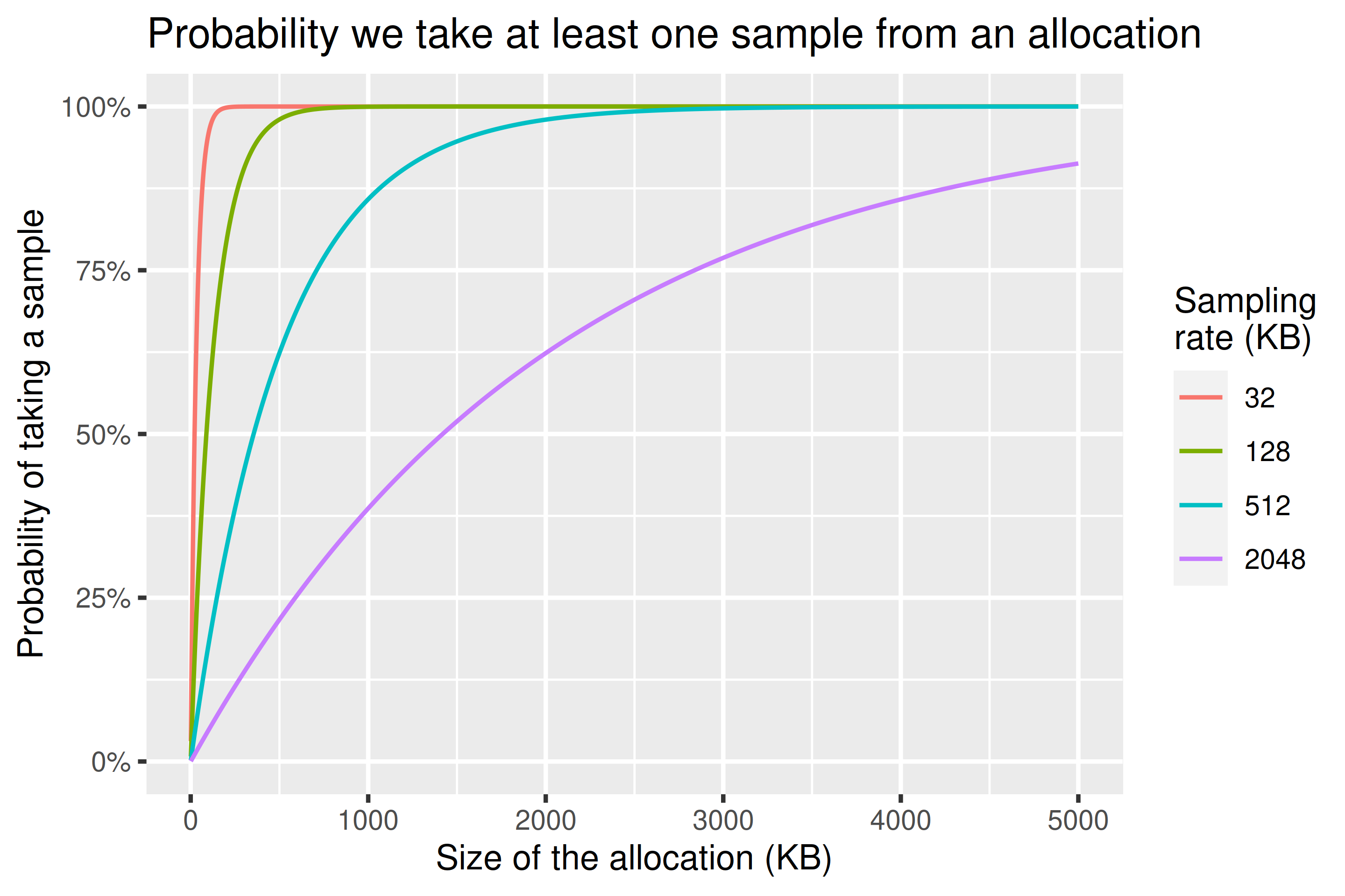
We can see from the chart below that if we 16X our sampling rate from 32KiB to 512KiB we still have a 95% chance of sampling anything above 1.5MiB. If we 64X it to 2048KiB we still have an 80% chance to sample anything above 3.5MiB.
Expected errors
We can also consider the expected error we’ll make at given allocation sizes and sampling rates. Like before it doesn’t matter where the allocation happens — if we have two allocations of the same type occurring at different times they have the same statistical properties as a single allocation with size equal to their sum. This is because the exponential distribution we use is memoryless.
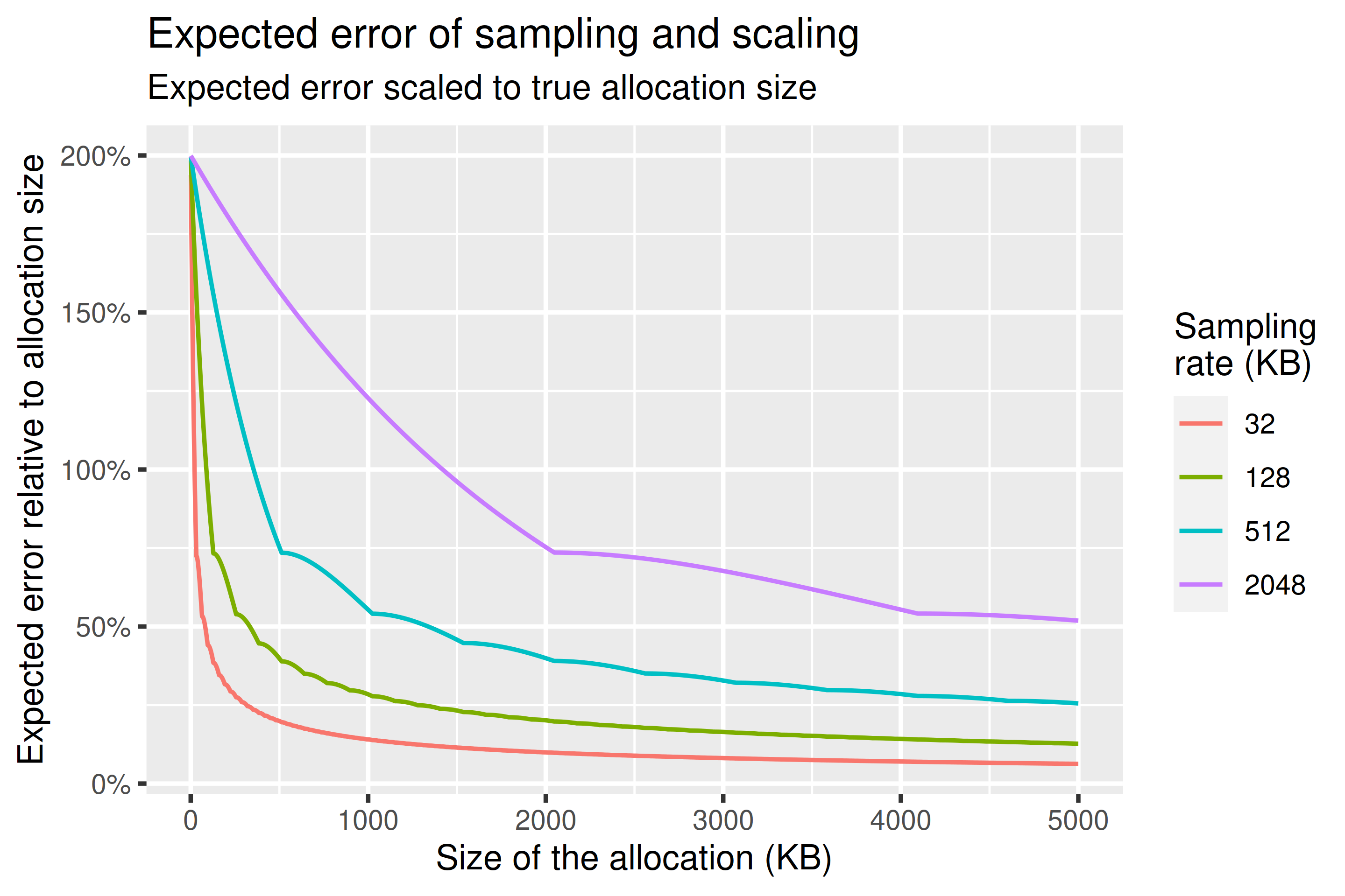
For expected error we report something like the mean absolute percentage error. This just means we see how wrong we might be in percent relative to the true allocation size, and then scale these results according to their probability of occurrence. This is an estimator that has some issues (i.e. it’s biased such that underestimates are more penalised) but it’s easy to reason about and it’s useful as a gauge of how wrong on average we might be with our estimates. I would recommend just reading this as analogous to a standard deviation.
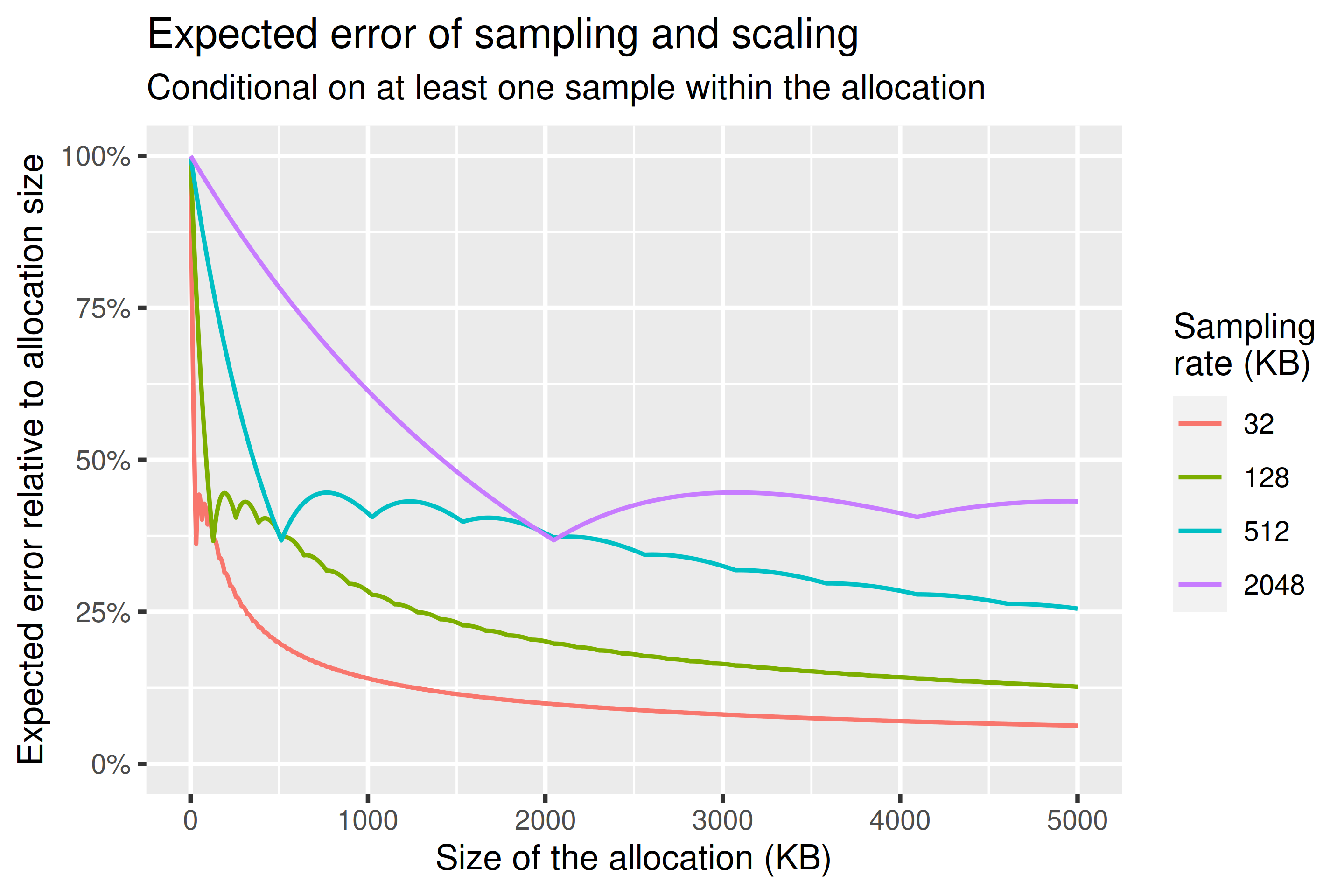
Charts below show both the expected error and the conditional expected error: the expected error assuming we have at least one sample within the allocation. There’s periodicity in both in line with the sampling rate used. The thing to take away is that, while the estimates are unbiased such that their expected value is equal to their real value, substantial errors are still possible.
Assuming that we take at least one sample of an allocation, what error might we expect? We can answer that using the following chart, which shows expected error conditional on at least one sample being taken. This is the expected error we can expect for the things that end up in our heap profile. It’s important to emphasise that this expected error methodology is not exact, and also that the underlying sampling remains unbiased — the expected value is the true value. This should be considered more as a measure akin to standard deviation.
Performance Considerations
STL Distributions
Benchmarking of the STL distributions on a Pixel 4 reinforces our approach of estimating the geometric distribution using an exponential distribution, as its performance is ~8x better (full results).
Draw sample from exponential distribution with p = 1 / 32000:
ARM64: 21.3ns (sd 0.066ns, negligibly small, smaller than a CPU cycle)
ARM32: 33.2ns (sd 0.011ns, negligibly small, smaller than a CPU cycle)
Draw sample from geometric distribution with p = 1 / 32000:
ARM64: 169ns (sd 0.023ns, negligibly small, smaller than a CPU cycle) (7.93x)
ARM32: 222ns (sd 0.118ns, negligibly small, smaller than a CPU cycle) (6.69x)
Appendix
Improvements made
We previously (before Android 12) returned the size of the allocation accurately and immediately if the allocation size was greater than our sampling rate. This had several impacts.
The most obvious impact is that with the old approach we would expect to sample an allocation equal in size to our sampling rate ~63% of the time, rather than 100%. This means there is a discontinuity in coverage between an allocation a byte smaller than our sampling rate, and one a byte larger. This is still unbiased from a statistical perspective, but it’s important to note.
Another unusual impact is that the sampling rate depends not only on the size of the memory being used, but also how it’s allocated. If our sampling rate were 10KB, and we have an allocation that’s 10KB, we sample it with certainty. If instead that 10KB is split among two 5KB allocations, we sample it with probability 63%. Again this doesn’t bias our results, but it means that our measurements of memory where there are many small allocations might be noisier than ones where there are a few large allocations, even if total memory used is the same. If we didn’t return allocations greater than the sampling rate every time, then the memorylessness property of the exponential distribution would mean our method is insensitive to how the memory is split amongst allocations, which seems a desirable property.
We altered the cutoff at which we simply returned the allocation size. Previously, as discussed, the cutoff was at the sampling rate, which led to a discontinuity. Now the cutoff is determined by the size at which we have a >99% chance of sampling an allocation at least once, given the sampling rate we’re using. This resolves the above issues.