
Getting Started with PerfettoSQL
PerfettoSQL is the foundation of trace analysis in Perfetto. It is a dialect of SQL that allows you to query the contents of your traces as if they were a database. This page introduces the core concepts of trace querying with PerfettoSQL and provides guidance on how to write queries.
Overview of Trace Querying
The Perfetto UI is a powerful tool for visual analysis, offering call stacks, timeline views, thread tracks, and slices. However, it also includes a robust SQL query language (PerfettoSQL) which is interpreted by a query engine (TraceProcessor) which allows you to extract data programmatically.
While the UI is powerful for myriad of analyses, users are able to write and execute queries within the Perfetto UI for multiple purposes such as:
- Extracting performance data from traces.
- Create custom visualizations (Debug tracks) to perform more complex analyses.
- Creating derived metrics.
- Identify performance bottlenecks using data-driven logic.
Beyond the Perfetto UI, you can query traces programmatically using the Python Trace Processor API or the C++ Trace Processor.
Perfetto also supports bulk trace analysis through the Batch Trace Processor. A key advantage of this system is query reusability: the same PerfettoSQL queries used for individual traces can be applied to large datasets without modification.
Core Concepts
Before writing queries, it's important to understand the foundational concepts of how Perfetto structures trace data.
Events
In the most general sense, a trace is simply a collection of timestamped "events". Events can have associated metadata and context which allows them to be interpreted and analyzed. Timestamps are in nanoseconds; the values themselves depend on the clock selected in TraceConfig.
Events form the foundation of trace processor and are one of two types: slices and counters.
Slices

A slice refers to an interval of time with some data describing what was happening in that interval. Some example of slices include:
- Atrace slices on Android
- Userspace slices from Chrome
Counters

A counter is a continuous value which varies over time. Some examples of counters include:
- CPU frequency for each CPU core
- RSS memory events - both from the kernel and polled from /proc/stats
- atrace counter events from Android
- Chrome counter events
Tracks
A track is a named partition of events of the same type and the same associated
context. A track associates events with a particular context such as a thread
(utid), process (upid), or CPU. For example:
- Sync userspace slices have one track for each thread which emitted an event
- Async userspace slices have one track for each "cookie" linking a set of async events
Tracks can be split into various types based on the type of event they contain and the context they are associated with. Examples include:
- Global tracks are not associated to any context and contain slices
- Thread tracks are associated to a single thread and contain slices
- Counter tracks are not associated to any context and contain counters
- CPU counter tracks are associated to a single CPU and contain counters
Note that the Perfetto UI also uses the term "tracks" to refer to the visual rows on the timeline. These are a UI-level concept for organizing the display and do not map 1:1 to trace processor tracks.
Scheduling
CPU scheduling data has its own dedicated tables and is not accessed through
tracks. The sched table contains one row for each time interval where a thread
was running on a CPU. Key columns include ts, dur, cpu, utid,
end_state, and priority.
For example, to see which threads were running on CPU 0:
SELECT ts, dur, utid
FROM sched
WHERE cpu = 0
LIMIT 10;
The complementary thread_state table shows what a thread was doing when it was
not running — whether it was sleeping, blocked in an uninterruptible sleep,
runnable and waiting for a CPU, and so on.
To query scheduling data with thread and process names, use the
sched.with_context stdlib module which provides the sched_with_thread_process
view:
INCLUDE PERFETTO MODULE sched.with_context;

SELECT ts, dur, cpu, thread_name, process_name
FROM sched_with_thread_process
WHERE thread_name = 'RenderThread'
LIMIT 10;
Stack sampling (CPU profiling)
Stack sampling periodically captures where code is executing, providing a statistical picture of CPU usage over time. Perfetto supports multiple data sources for this, including Linux perf, simpleperf, macOS Instruments, and Chrome CPU profiling.
The raw data lives in source-specific tables (perf_sample,
cpu_profile_stack_sample). Each sample has a callsite_id which points into
the stack_profile_callsite table — a linked list of frames forming the
callstack. Each callsite row has a frame_id pointing to stack_profile_frame
(the function name and mapping/binary) and a parent_id pointing to the next
frame up the stack.
To resolve a sample to its leaf (most recent) frame, join through callsite to frame:
SELECT
  s.ts,
  s.utid,
  f.name AS function_name,
  m.name AS binary_name
FROM perf_sample AS s
JOIN stack_profile_callsite AS c ON s.callsite_id = c.id
JOIN stack_profile_frame AS f ON c.frame_id = f.id
JOIN stack_profile_mapping AS m ON f.mapping = m.id
LIMIT 10;
For aggregation and summary across full callstacks, use the
stacks.cpu_profiling stdlib module. It provides a unified
cpu_profiling_samples table across all data sources and a
cpu_profiling_summary_tree table that computes self counts (samples where the
function was the leaf frame) and cumulative counts (samples where the function
appeared anywhere in the callstack):
INCLUDE PERFETTO MODULE stacks.cpu_profiling;

-- Unified samples across all CPU profiling data sources:
SELECT ts, thread_name, callsite_id
FROM cpu_profiling_samples
LIMIT 10;

-- Aggregated callstack tree with self and cumulative counts:
SELECT name, mapping_name, self_count, cumulative_count
FROM cpu_profiling_summary_tree
ORDER BY cumulative_count DESC
LIMIT 20;
Heap profiling
Heap profiling captures memory allocations along with their callstacks, showing where memory is being allocated (and freed) over time. This is useful for finding memory leaks and understanding allocation patterns.
The heap_profile_allocation table contains one row per allocation or free
event. Key columns include ts, upid, callsite_id, count, and size.
The upid column can be joined to the process table to get the full process
command line (cmdline) and real pid.
SELECT ts, upid, size, count
FROM heap_profile_allocation
WHERE size > 0
ORDER BY size DESC
LIMIT 10;
Like CPU profiling, each allocation has a callsite_id pointing into the
callstack tables. To resolve an allocation to its leaf frame:
SELECT
  a.ts,
  a.size,
  f.name AS function_name,
  m.name AS binary_name
FROM heap_profile_allocation AS a
JOIN stack_profile_callsite AS c ON a.callsite_id = c.id
JOIN stack_profile_frame AS f ON c.frame_id = f.id
JOIN stack_profile_mapping AS m ON f.mapping = m.id
WHERE a.size > 0
LIMIT 10;
For full callstack aggregation with self and cumulative sizes, use the
android.memory.heap_profile.summary_tree stdlib module:
INCLUDE PERFETTO MODULE android.memory.heap_profile.summary_tree;

SELECT name, mapping_name, self_size, cumulative_size
FROM android_heap_profile_summary_tree
ORDER BY cumulative_size DESC
LIMIT 20;
Heap graph (heap dumps)
Heap graph data captures a snapshot of the managed heap (e.g., Java/ART on Android), recording the full object reference graph at a point in time. This is useful for understanding memory retention and finding leaks in managed runtimes.
Key tables include:
heap_graph_object: objects on the heap, with their type, size, and reachability information.heap_graph_reference: references between objects (which object points to which).heap_graph_class: class metadata (name, superclass, classloader).
SELECT
  c.name AS class_name,
  SUM(o.self_size) AS total_size,
  COUNT() AS object_count
FROM heap_graph_object AS o
JOIN heap_graph_class AS c ON o.type_id = c.id
WHERE o.reachable
GROUP BY c.name
ORDER BY total_size DESC
LIMIT 10;
Thread and process identifiers
The handling of threads and processes needs special care when considered in the
context of tracing; identifiers for threads and processes (e.g. pid/tgid and
tid in Android/macOS/Linux) can be reused by the operating system over the
course of a trace. This means they cannot be relied upon as a unique identifier
when querying tables in trace processor.
To solve this problem, the trace processor uses utid (unique tid) for
threads and upid (unique pid) for processes. All references to threads and
processes (e.g. in CPU scheduling data, thread tracks) uses utid and upid
instead of the system identifiers.
Querying traces in the Perfetto UI
Now that you understand the core concepts, you can start writing queries.
Perfetto provides two ways to explore trace data directly in the UI:
- The Data Explorer page lets you browse available tables interactively without writing SQL. This is useful for discovering what data is in your trace and understanding table schemas.
- The Query (SQL) tab provides a free-form SQL editor for writing and executing PerfettoSQL queries.
To use the Query tab:
Open a trace in the Perfetto UI.
Click the Query (SQL) tab in the navigation bar (see image below).
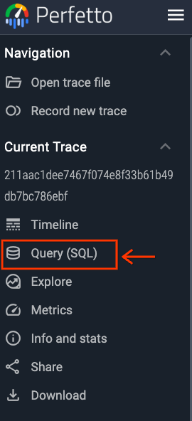
Upon selecting this tab, the querying UI will show up and you will be able to free-form write your PerfettoSQL queries, it will let you write queries, show query results and query history as shown in the image below.

- Enter your query in the Query UI area and press Ctrl + Enter (or Cmd + Enter) to execute.
Once executed query results will be shown within the same window.
This method of querying is useful when you have some degree of knowledge about how and what to query.
In order to find out how to write queries refer to the Syntax guide, then in order to find available tables, modules, functions, etc. refer to the Standard Library.
A lot of times, it will be useful to transform query results into tracks to perform complex analyses within the UI, we encourage readers to take a look at Debug Tracks for more information on how to achieve this.
Example: Executing a basic query
The simplest way to explore a trace is to select from the raw tables. For example, to see the first 10 slices in a trace, you can run:
SELECT ts, dur, name FROM slice LIMIT 10;Which you can write and execute by clicking on Run Query within the PerfettoSQL querying UI, below is an example from a trace.

Adding Context to Slices
A common question when querying slices is: "how do I get the thread or process
that emitted this slice?" The easiest way is to use the slices.with_context
standard library module, which provides pre-joined views that include thread and
process information directly.
INCLUDE PERFETTO MODULE slices.with_context;Once imported, you have access to three views:
thread_slice — slices from thread tracks, with thread and process context:
SELECT ts, dur, name, thread_name, process_name, tid, pid
FROM thread_slice
WHERE name = 'measure';
process_slice — slices from process tracks, with process context:
SELECT ts, dur, name, process_name, pid
FROM process_slice
WHERE name LIKE 'MyEvent%';
thread_or_process_slice — a combined view of both thread and process
slices, useful when you want to search across all slices regardless of track
type:
SELECT ts, dur, name, thread_name, process_name
FROM thread_or_process_slice
WHERE dur > 1000000;
These views are the recommended approach for most slice queries. They handle
the joins for you and expose commonly needed columns like thread_name,
process_name, tid, pid, utid, and upid.
Manual JOINs for more control
Under the hood, thread_slice joins slice with thread_track, thread, and
process. If you need columns not exposed by the stdlib views, or if you're
working with tables that don't have a stdlib convenience view (e.g., counter
tracks), you can write the joins yourself.
The thread and process tables map utids and upids to the system-level
tid, pid, and names:
SELECT tid, name
FROM thread
WHERE utid = 10;
For example, to get upids of processes with a mem.swap counter greater
than 1000:
SELECT upid
FROM counter
JOIN process_counter_track ON process_counter_track.id = counter.track_id
WHERE process_counter_track.name = 'mem.swap' AND value > 1000;
Or to manually join slices with thread info:
SELECT thread.name AS thread_name
FROM slice
JOIN thread_track ON slice.track_id = thread_track.id
JOIN thread USING(utid)
WHERE slice.name = 'measure'
GROUP BY thread_name;
Best Practices
Prefer stdlib views over manual JOINs
The standard library provides pre-joined views for the most common queries.
Using thread_slice, process_slice, thread_or_process_slice, and
sched_with_thread_process saves boilerplate and avoids mistakes in join
conditions.
Filter early
Always place WHERE clauses — especially filters on name — as early as
possible. This lets trace processor skip scanning rows that won't contribute
to the result.
Use LIMIT when exploring
When you're unfamiliar with a table, start with a small query to understand its shape before writing anything complex:
SELECT * FROM slice LIMIT 10;Timestamps are in nanoseconds
All ts and dur values are in nanoseconds. For human-readable output, use the
time.conversion stdlib module:
INCLUDE PERFETTO MODULE time.conversion;

SELECT name, time_to_ms(dur) AS dur_ms
FROM slice
WHERE dur > time_from_ms(10);
Advanced Querying
For users who need to go beyond the standard library or build their own abstractions, PerfettoSQL provides several advanced features.
Helper functions
Helper functions are functions built into C++ which reduce the amount of boilerplate which needs to be written in SQL.
Extract args
EXTRACT_ARG is a helper function which retrieves a property of an event (e.g.
slice or counter) from the args table.
It takes an arg_set_id and key as input and returns the value looked up in
the args table.
For example, to retrieve the prev_comm field for sched_switch events in the
ftrace_event table.
SELECT EXTRACT_ARG(arg_set_id, 'prev_comm')
FROM ftrace_event
WHERE name = 'sched_switch'
Behind the scenes, the above query would desugar to the following:
SELECT
  (
    SELECT string_value
    FROM args
    WHERE key = 'prev_comm' AND args.arg_set_id = raw.arg_set_id
  )
FROM ftrace_event
WHERE name = 'sched_switch'
Operator tables
SQL queries are usually sufficient to retrieve data from trace processor. Sometimes though, certain constructs can be difficult to express pure SQL.
In these situations, trace processor has special "operator tables" which solve a particular problem in C++ but expose an SQL interface for queries to take advantage of.
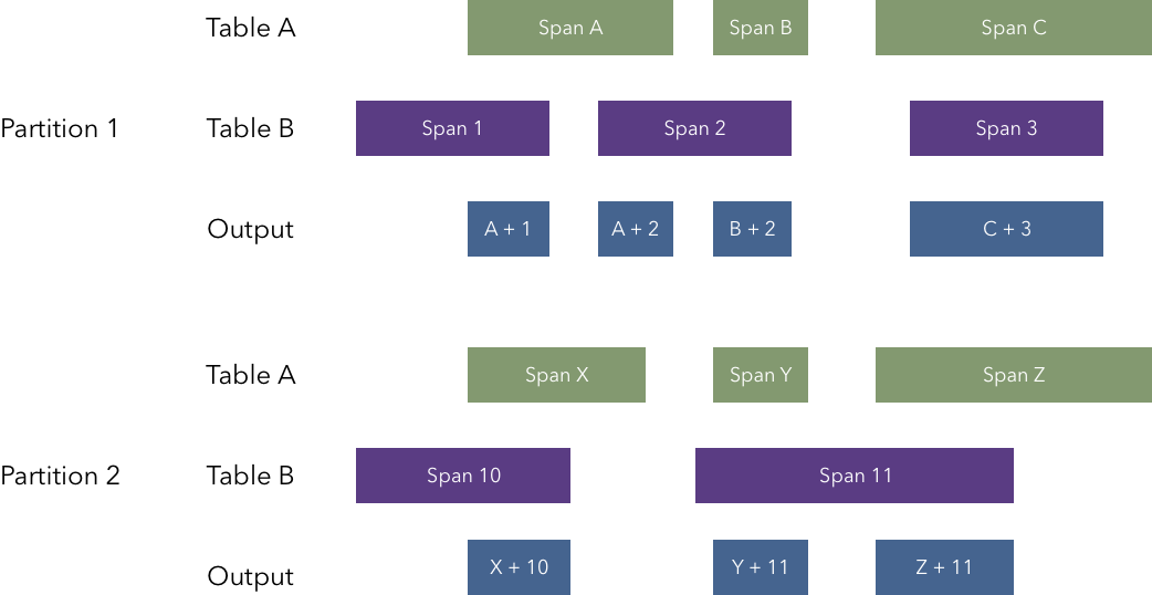
Span join
Span join is a custom operator table which computes the intersection of spans of time from two tables or views. A span in this concept is a row in a table/view which contains a "ts" (timestamp) and "dur" (duration) columns.
A column (called the partition) can optionally be specified which divides the rows from each table into partitions before computing the intersection.
-- Get all the scheduling slices
CREATE VIEW sp_sched AS
SELECT ts, dur, cpu, utid
FROM sched;

-- Get all the cpu frequency slices
CREATE VIEW sp_frequency AS
SELECT
  ts,
  lead(ts) OVER (PARTITION BY track_id ORDER BY ts) - ts as dur,
  cpu,
  value as freq
FROM counter
JOIN cpu_counter_track ON counter.track_id = cpu_counter_track.id
WHERE cpu_counter_track.name = 'cpufreq';

-- Create the span joined table which combines cpu frequency with
-- scheduling slices.
CREATE VIRTUAL TABLE sched_with_frequency
USING SPAN_JOIN(sp_sched PARTITIONED cpu, sp_frequency PARTITIONED cpu);

-- This span joined table can be queried as normal and has the columns from both
-- tables.
SELECT ts, dur, cpu, utid, freq
FROM sched_with_frequency;
NOTE: A partition can be specified on neither, either or both tables. If specified on both, the same column name has to be specified on each table.
WARNING: An important restriction on span joined tables is that spans from the same table in the same partition cannot overlap. For performance reasons, span join does not attempt to detect and error out in this situation; instead, incorrect rows will silently be produced.
WARNING: Partitions mush be integers. Importantly, string partitions are not
supported; note that strings can be converted to integers by applying the
HASH function to the string column.
Left and outer span joins are also supported; both function analogously to the left and outer joins from SQL.
-- Left table partitioned + right table unpartitioned.
CREATE VIRTUAL TABLE left_join
USING SPAN_LEFT_JOIN(table_a PARTITIONED a, table_b);

-- Both tables unpartitioned.
CREATE VIRTUAL TABLE outer_join
USING SPAN_OUTER_JOIN(table_x, table_y);
NOTE: there is a subtlety if the partitioned table is empty and is either a) part of an outer join b) on the right side of a left join. In this case, no slices will be emitted even if the other table is non-empty. This approach was decided as being the most natural after considering how span joins are used in practice.
Ancestor slice
Given a slice, ancestor_slice returns all slices on the same track that are
direct parents above it (i.e. all slices found by following the parent_id
chain up to the root at depth 0).
+----------------------------+  depth 0  \
| A (id=1)                   |            |
| +------------+ +--------+  |            | ancestor_slice(4)
| | B (id=2)   | | D      |  |  depth 1   > returns A, B
| | +--------+ | |        |  |            |
| | |C (id=4)| | |        |  |  depth 2  /
| | +--------+ | |        |  |
| +------------+ +--------+  |
+----------------------------+
The returned format is the same as the slice table.
For example, the following finds the top-level slice for each slice of interest:
CREATE VIEW interesting_slices AS
SELECT id, ts, dur, track_id
FROM slice WHERE name LIKE "%interesting slice name%";

SELECT
  *
FROM
  interesting_slices LEFT JOIN
  ancestor_slice(interesting_slices.id) AS ancestor ON ancestor.depth = 0
TIP: To check if one slice is an ancestor of another without fetching all
ancestors, use the slice_is_ancestor(ancestor_id, descendant_id) function
which is available without any imports.
Descendant slice
Given a slice, descendant_slice returns all slices on the same track that are
nested under it (i.e. all slices at a greater depth within the same time range).
+----------------------------+  depth 0
| A (id=1)                   |
| +------------+ +--------+  |           \
| | B (id=2)   | | D      |  |  depth 1   |
| | +--------+ | | +----+ |  |            | descendant_slice(1)
| | |C (id=4)| | | | E  | |  |  depth 2   > returns B, C, D, E
| | +--------+ | | +----+ |  |            |
| +------------+ +--------+  |           /
+----------------------------+
The returned format is the same as the slice table.
For example, the following finds the number of slices under each slice of interest:
CREATE VIEW interesting_slices AS
SELECT id, ts, dur, track_id
FROM slice WHERE name LIKE "%interesting slice name%";

SELECT
  interesting_slices.*,
  (
    SELECT COUNT(*)
    FROM descendant_slice(interesting_slices.id)
  ) AS total_descendants
FROM interesting_slices
Connected/Following/Preceding flows
DIRECTLY_CONNECTED_FLOW, FOLLOWING_FLOW and PRECEDING_FLOW are custom operator tables that take a slice table's id column and collect all entries of flow table, that are directly or indirectly connected to the given starting slice.
DIRECTLY_CONNECTED_FLOW(start_slice_id) - contains all entries of
flow table that are present in any
chain of kind: flow[0] -> flow[1] -> ... -> flow[n], where
flow[i].slice_out = flow[i+1].slice_in and
flow[0].slice_out = start_slice_id OR start_slice_id = flow[n].slice_in.
NOTE: Unlike the following/preceding flow functions, this function will not include flows connected to ancestors or descendants while searching for flows from a slice. It only includes the slices in the directly connected chain.
FOLLOWING_FLOW(start_slice_id) - contains all flows which can be reached from
a given slice via recursively following from flow's outgoing slice to its
incoming one and from a reached slice to its child. The return table contains
all entries of flow table that are
present in any chain of kind: flow[0] -> flow[1] -> ... -> flow[n], where
flow[i+1].slice_out IN DESCENDANT_SLICE(flow[i].slice_in) OR flow[i+1].slice_out = flow[i].slice_in
and
flow[0].slice_out IN DESCENDANT_SLICE(start_slice_id) OR flow[0].slice_out = start_slice_id.
PRECEDING_FLOW(start_slice_id) - contains all flows which can be reached from
a given slice via recursively following from flow's incoming slice to its
outgoing one and from a reached slice to its parent. The return table contains
all entries of flow table that are
present in any chain of kind: flow[n] -> flow[n-1] -> ... -> flow[0], where
flow[i].slice_in IN ANCESTOR_SLICE(flow[i+1].slice_out) OR flow[i].slice_in = flow[i+1].slice_out
and
flow[0].slice_in IN ANCESTOR_SLICE(start_slice_id) OR flow[0].slice_in = start_slice_id.
--number of following flows for each slice
SELECT (SELECT COUNT(*) FROM FOLLOWING_FLOW(slice_id)) as following FROM slice;
Next Steps
Now that you have a foundational understanding of PerfettoSQL, you can explore the following topics to deepen your knowledge:
- PerfettoSQL Syntax: Learn about the SQL syntax supported by Perfetto, including special features for creating functions, tables, and views.
- Standard Library: Explore the rich set of modules available in the standard library for analyzing common scenarios like CPU usage, memory, and power.
- Trace Processor (C++): Learn how to use the interactive shell and the underlying C++ library.
- Trace Processor (Python): Leverage the Python API to combine trace analysis with the rich data science and visualization ecosystem.